ModelingToolkit.jl：面向科学计算和机器学习的高性能Julia符号-数值计算建模框架

Python 机器学习

访问GitHub主页

共317Star

详细介绍

ModelingToolkit.jl

ModelingToolkit.jl is a modeling framework for high-performance symbolic-numeric computation in scientific computing and scientific machine learning. It allows for users to give a high-level description of a model for symbolic preprocessing to analyze and enhance the model. ModelingToolkit can automatically generate fast functions for model components like Jacobians and Hessians, along with automatically sparsifying and parallelizing the computations. Automatic transformations, such as index reduction, can be applied to the model to make it easier for numerical solvers to handle.

For information on using the package, see the stable documentation. Use the in-development documentation for the version of the documentation which contains the unreleased features.

High-Level Examples

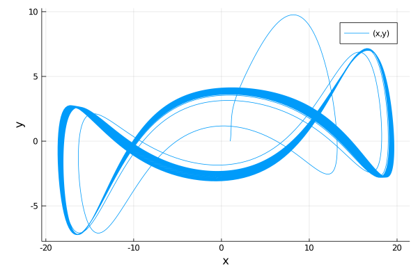
First, let's define a second order riff on the Lorenz equations, symbolically lower it to a first order system, symbolically generate the Jacobian function for the numerical integrator, and solve it.

using ModelingToolkit, OrdinaryDiffEq

@parameters t σ ρ β
@variables x(t) y(t) z(t)
@derivatives D'~t

eqs = [D(D(x)) ~ σ*(y-x),
       D(y) ~ x*(ρ-z)-y,
       D(z) ~ x*y - β*z]

sys = ODESystem(eqs)
sys = ode_order_lowering(sys)

u0 = [D(x) => 2.0,
      x => 1.0,
      y => 0.0,
      z => 0.0]

p  = [σ => 28.0,
      ρ => 10.0,
      β => 8/3]

tspan = (0.0,100.0)
prob = ODEProblem(sys,u0,tspan,p,jac=true)
sol = solve(prob,Tsit5())
using Plots; plot(sol,vars=(x,y))

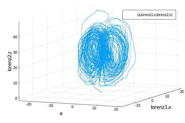
This automatically will have generated fast Jacobian functions, making it more optimized than directly building a function. In addition, we can then use ModelingToolkit to compose multiple ODE subsystems. Now, let's define two interacting Lorenz equations and simulate the resulting Differential-Algebraic Equation (DAE):

using ModelingToolkit, OrdinaryDiffEq

@parameters t σ ρ β
@variables x(t) y(t) z(t)
@derivatives D'~t

eqs = [D(x) ~ σ*(y-x),
       D(y) ~ x*(ρ-z)-y,
       D(z) ~ x*y - β*z]

lorenz1 = ODESystem(eqs,name=:lorenz1)
lorenz2 = ODESystem(eqs,name=:lorenz2)

@variables a
@parameters γ
connections = [0 ~ lorenz1.x + lorenz2.y + a*γ]
connected = ODESystem(connections,t,[a],[γ],systems=[lorenz1,lorenz2])

u0 = [lorenz1.x => 1.0,
      lorenz1.y => 0.0,
      lorenz1.z => 0.0,
      lorenz2.x => 0.0,
      lorenz2.y => 1.0,
      lorenz2.z => 0.0,
      a => 2.0]

p  = [lorenz1.σ => 10.0,
      lorenz1.ρ => 28.0,
      lorenz1.β => 8/3,
      lorenz2.σ => 10.0,
      lorenz2.ρ => 28.0,
      lorenz2.β => 8/3,
      γ => 2.0]

tspan = (0.0,100.0)
prob = ODEProblem(connected,u0,tspan,p)
sol = solve(prob,Rodas5())

using Plots; plot(sol,vars=(a,lorenz1.x,lorenz2.z))

推荐源码